Standard workflow with restricted cubic splines • rmsMD

library(rms)
library(rmsMD)

Introduction

The modelsummary_rms function is designed to process output from models fitted using the rms package and generate a summarised dataframe of the results. The goal is to produce publication-ready summaries of the models. The ggrmsMD function generates publication ready plots of variables modelled with restricted cubic splines.

This vignette will guide you through the basic usage of the functions on a model including restricted cubic splines.

Installation and Setup

For these vignettes we will use a simulated dataset to predict the impact of age, BMI, Sex and Smoking status on outcome after surgery. The models are for illustration purposes only. Note, if you plan to output the results into Microsoft Word, we recommend also installing flextable and officer.

# Load in the simulated data
data <- simulated_rmsMD_data()

# Set the datadist which is required for rms modelling 
# (these two lines are standard)
dd <- datadist(data)    
options(datadist='dd')

Fitting Model with Restricted Cubic Splines

Restricted Cubic Splines (RCS) are a flexible modelling tool used to capture non-linear relationships between predictors and outcomes. In medicine, for the majority of continuous variables (e.g. age, blood pressure, or biomarker levels) the assumption of linearity may not hold. A key highlight of the rms package is the ability to analyse variables using RCS.

The rmsMD package is designed to report and summarise models that include RCS terms. Here is an example model predicting occurrence of complications after surgery (binary), with the continuous variables age and BMI modelled using restricted cubic splines with 4 knots:

# Fit an OLS model including a restricted cubic spline 
# for Age and BMI (with 4 knots)
fit_lrm <- lrm(majorcomplication ~ 
                 rcs(age,4) + 
                 rcs(bmi,4) + 
                 sex + 
                 smoking, 
               data = data,
               x = TRUE, y = TRUE)
# setting x = TRUE, y = TRUE allows subsequent likelihood ratio tests to be 
# performed which is recommended for lrm() and cph() models

Intuitive output with modelsummary_rms

Individual coefficients for RCS terms are difficult to interpret in isolation. Instead, an overall p-value can be generated to assess whether the overall relationship between the RCS variable and outcome is significant. By default modelsummary_rms removes the individual RCS coefficients, replacing them with the overall p-value for that variable.

# Generate an rmsMD model summary using default settings
modelsummary_rms(fit_lrm)
#>           variable                OR_95CI Pvalue
#> 1       sex=Female                    Ref      -
#> 2         sex=Male 1.078 (0.927 to 1.255)  0.330
#> 3    smoking=Never                    Ref      -
#> 4   smoking=Former 0.986 (0.806 to 1.207)  0.892
#> 5  smoking=Current 2.078 (1.731 to 2.496) <0.001
#> 6 RCSoverallP: age                LR test <0.001
#> 7 RCSoverallP: bmi                LR test  0.034

# Outputting this as a table
knitr::kable(modelsummary_rms(fit_lrm))

variable	OR_95CI	Pvalue
sex=Female	Ref	-
sex=Male	1.078 (0.927 to 1.255)	0.330
smoking=Never	Ref	-
smoking=Former	0.986 (0.806 to 1.207)	0.892
smoking=Current	2.078 (1.731 to 2.496)	<0.001
RCSoverallP: age	LR test	<0.001
RCSoverallP: bmi	LR test	0.034

P values for restricted cubic spline terms in these outputs indicate whether there is an association between the predictor and outcome. Please note that this association can be either linear or non-linear. The P value reflects the presence of an association, not its shape. We recommend that these associations are then plotted using the ggrmsMD function, shown below, to assess the nature of these relationships.

Plotting with ggrmsMD

Now that the model and overall p values have been assessed, the ggrmsMD function from rmsMD can be used to assess the relationship between variables modelled with restricted cubic splines, and the outcome.

As a minimum, the model fit and data should be passed into the function. ggrmsMD will then generate plots for all variables which were modelled with restricted cubic splines. The default behavior is to plot: predicted outcome for linear regression models, adjusted OR for logistic regression, and adjusted HR for Cox regression. All of these plots are adjusted for all other variables in the model.

Here is the most basic use case with the logistic regression model for post-operative complications above:

# Most basic output
ggrmsMD(fit_lrm, data)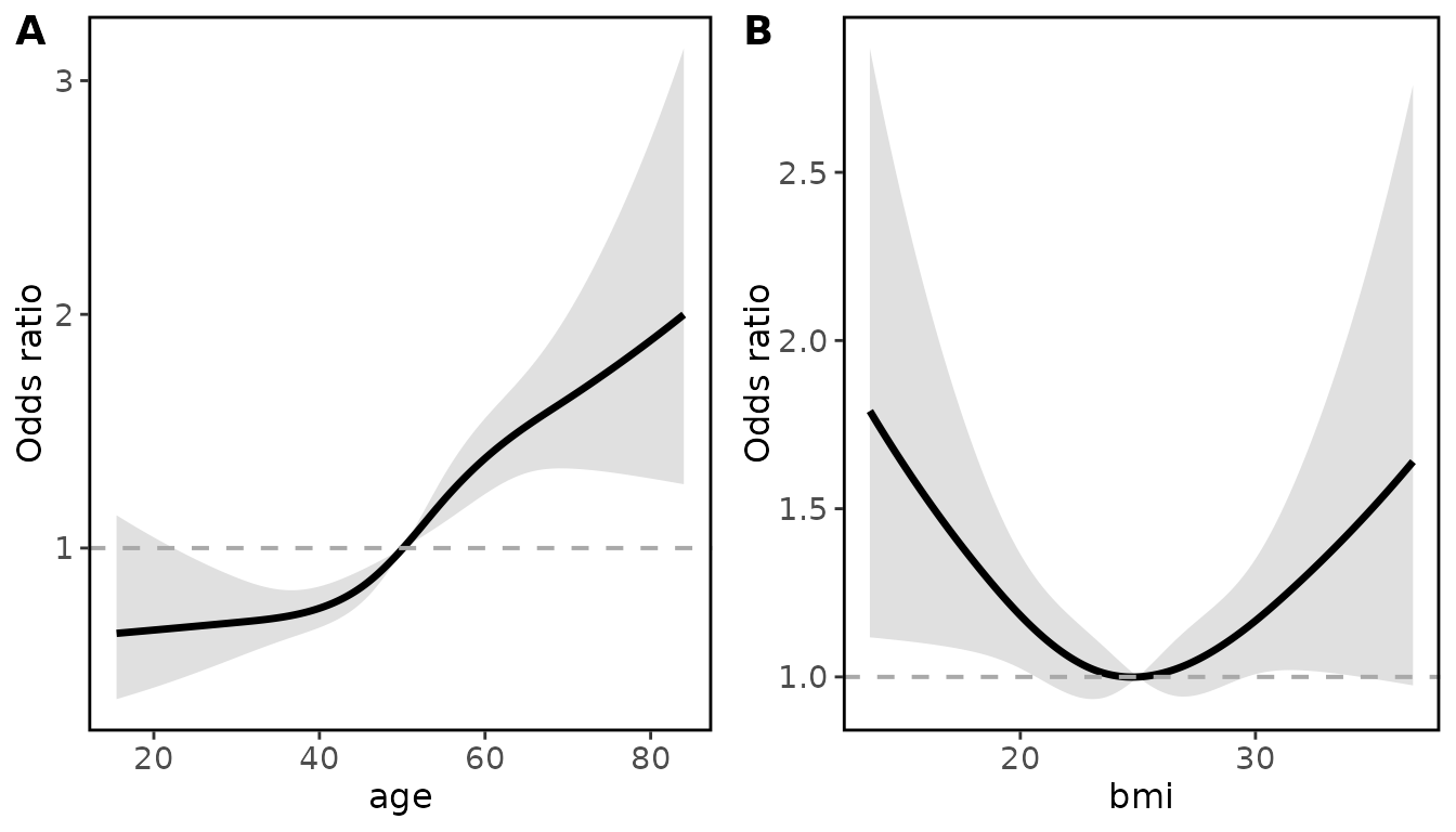

Further arguments in ggrmsMD allow these plots to be editted into a publication ready format. Example of a publication ready plot:

# x axis labels can be stored in a list
xlabels <- list ("age" = "Age (years)",
                 "bmi" = "Body Mass Index")

# titles for each variable can be stored in a list
titles <- list ("age" = "Impact of Age on Complications",
                 "bmi" = "Impact of BMI on Complications")

ggrmsMD(fit_lrm, data,
        # set y axis label for all plots
        ylab = "Complications (adjusted OR)", 
        # set y axis limits
        ylim = c(0,3),
        # set higher OR as inferior outcome to assign red shading
        shade_inferior = "higher", 
        # set x axis labels for each variable
        xlabs = xlabels, 
        # set titles for each variable
        titles = titles 
        )

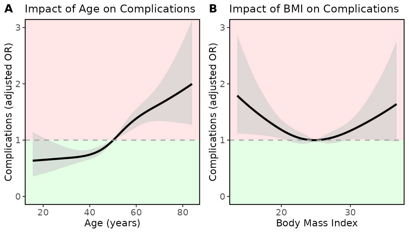
Further arguments allow for log transformation of axes, selection of which variables are included, option to output plot lists rather than combined plots, ability to plot predicted probability rather than OR, etc. For further details please see the vignette Further_details_ggrmsMD. Outputted plots are ggplots, and therefore can be further adapted using that framework.

Exporting to Microsoft Word

The output of modelsummary_rms is a dataframe, as this is easy to work with and further process if required. This dataframe output can easily be exported to a word document using flextable and officer packages.

library(officer)
library(flextable)
library(dplyr)
#> 
#> Attaching package: 'dplyr'
#> The following objects are masked from 'package:Hmisc':
#> 
#>     src, summarize
#> The following objects are masked from 'package:stats':
#> 
#>     filter, lag
#> The following objects are masked from 'package:base':
#> 
#>     intersect, setdiff, setequal, union

# Convert modelsummary_rms dataframe to a flextable
rmsMD_as_table <- flextable(modelsummary_rms(fit_lrm))

# Create a new Word document, add table and a heading
doc <- read_docx() %>%
  body_add_flextable(rmsMD_as_table) %>%
  body_add_par("Model summary from rmsMD", style = "heading 2")

# Temporary file path for output (replace with your actual path as needed)
output_path <- file.path(tempdir(), "example_output.docx")

# Generate the Word document
print(doc, target = output_path)

# Alternatively, save as 'temp.docx' in the working directory
print(doc, target = "temp.docx")